Umgang mit zwei axis-Umgebungen

schlenzer · Beitrag von **schlenzer** » Mo 20. Jul 2015, 23:39

Guten Abend,

ich bin dabei meine Diplomarbeit zu schreiben und benötige euere Hilfe!
Ich habe zwei axis-Umgebungen, in denen unterschiedliche Zusammenhänge geplottet werden. Die x-Koordinaten sind bei beiden Diagrammen gleich. Ich würde gerne im unteren Diagramm die Fläche unterhalb der Kurve bis zum Schnittpunkt (x-Koordinate) zweier Linien aus dem oberen Diagramm farbig markieren.

\documentclass[a4paper]{scrreprt}	

\usepackage{tikz}
%pdfplots
\usepackage{pgfplots}
\usepgfplotslibrary{fillbetween}
\usetikzlibrary{intersections}
\usetikzlibrary{calc}

\begin{document}
\begin{tikzpicture}
\begin{axis}[%
name=plot1,
scale only axis,
width=13cm,
height=5cm,
]%
\addplot [
color=blue,
solid
]
coordinates{
	(0,0)(2,2)(4,4)(6,6)
};
\draw[red, dashed, thick](axis cs:1,2) -- (axis cs:3,2);
\end{axis}
\begin{axis}[%
at=(plot1.below south west), anchor=above north west,
scale only axis,
width=13cm,
height=5cm,
]%
\addplot [
color=blue,
solid
]
coordinates{
	(0,0)(1,2)(2,4)(5,6)
};
\end{axis}
\end{tikzpicture}
\end{document}

Vielen Dank für euere Hilfe!
MFG

sudo · Beitrag von **sudo** » Di 21. Jul 2015, 09:39

Ich bin mir nicht sicher, ob ich dich und deine Plot verstehe, aber hier ist ein Vorschlag.

\documentclass[a4paper]{scrreprt}   

\usepackage{tikz}
%pdfplots
\usepackage{pgfplots}
\usepgfplotslibrary{fillbetween}
\usetikzlibrary{intersections}
\usetikzlibrary{calc}

\begin{document}
\begin{tikzpicture}
\begin{axis}[%
name=plot1,
scale only axis,
width=13cm,
height=5cm,
]%
\addplot [
color=blue,
solid
]
coordinates{
   (0,0)(2,2)(4,4)(6,6)
};
\draw[red, dashed, thick](axis cs:1,2) -- (axis cs:3,2);
\end{axis}
\begin{axis}[%
at=(plot1.below south west), anchor=above north west,
scale only axis,
width=13cm,
height=5cm,
]%
\addplot [
color=blue,
solid, name path global = myFunction
]
coordinates{
   (0,0)(1,2)(2,4)(5,6)
};
\fill[blue, fill opacity=0.05]  (axis cs:0,0) --  (axis cs:2,2) --  (axis cs:2,0) -- cycle;  
\end{axis}
\end{tikzpicture}
\end{document}

esdd · Beitrag von **esdd** » Di 21. Jul 2015, 10:18

Ich würde zunächst dafür sorgen, dass beide x-Achsen wirklich gleich eingeteilt sind. Und auch dann funktioniert das folgende nur, wenn die Plots auch vertikal aneinander ausgerichtet sind:

\documentclass[a4paper]{scrreprt}   
\usepackage{pgfplots}
\pgfplotsset{compat=1.12} 
\usepgfplotslibrary{fillbetween} 
\usetikzlibrary{intersections} 
\begin{document} 
\begin{tikzpicture}[
  /pgfplots/every axis/.style={%
    scale only axis, 
    width=13cm, 
    height=5cm,
    xmin=-.5,xmax=6.5,
    enlarge y limits=upper
  }
]
\begin{axis}[name=plot1]% 
  \addplot [ 
      color=blue, 
      solid,
      name path=A
    ] 
    coordinates{ 
        (0,0)(2,2)(4,4)(6,6) 
    }; 
  \draw[red, dashed, thick,name path=B](axis cs:1,2) -- (axis cs:3,2);
  \path[name intersections={of=A and B, by=C}];
\end{axis} 

\begin{axis}[% 
  at=(plot1.below south west), anchor=above north west, 
]% 
  \addplot [ 
      color=blue, 
      solid,
      name path=A 
    ] 
    coordinates{ 
      (0,0)(1,2)(2,4)(5,6) 
    };
  \path [name path=B]
    (\pgfkeysvalueof{/pgfplots/xmin},0)--(\pgfkeysvalueof{/pgfplots/xmax},0);
  \addplot[purple!10]fill between[
    of= A and B,
    soft clip={(\pgfkeysvalueof{/pgfplots/xmin},\pgfkeysvalueof{/pgfplots/ymin})rectangle(C|-current axis.north)}
    ];
\end{axis}
\draw[dashed,thin](C)--(C|-current axis.south);
\end{tikzpicture} 
\end{document}

Gruß
Elke

Bild

schlenzer · Beitrag von **schlenzer** » Di 21. Jul 2015, 23:22

Danke für euere schnelle Antwort. Für dieses Beispiel hat es ja super geklappt, ersetzte ich jedoch die Koordinaten aus den Minibeispiel mit den echten Daten, so funktioniert das ganze leider nicht mehr. Das Problem liegt darin, dass die Kurve keine geometrische Form hat.
Hier nochmal das Mini-Beispiel mit meinen Daten und den Vorschlag von Elke.

\documentclass[a4paper]{scrreprt}  
\usepackage{pgfplots}
\pgfplotsset{compat=1.12}
\usepgfplotslibrary{fillbetween}
\usetikzlibrary{intersections}
\begin{document}
\begin{tikzpicture}[
  /pgfplots/every axis/.style={%
    scale only axis,
    width=13cm,
    height=5cm,
    xmin=-.5,xmax=6.5,
    enlarge y limits=upper
  }
]
\begin{axis}[name=plot1]%
  \addplot [
      color=blue,
      solid,
      name path=A
    ]
    coordinates{
    	(0.105,0)(0.11,11.9866)(0.115,36.5101)(0.12,61.0337)(0.125,85.5572)(0.13,110.081)(0.135,134.604)(0.14,159.128)(0.145,183.651)(0.15,208.175)(0.155,232.699)(0.16,257.222)(0.165,281.746)(0.17,306.269)(0.175,330.793)(0.18,355.316)(0.185,379.84)(0.19,404.363)(0.195,428.887)(0.2,453.41)(0.205,477.934)(0.21,502.458)(0.215,526.981)(0.22,551.505)(0.225,578.131)(0.23,607.435)(0.235,636.738)(0.24,666.042)(0.245,696.76)(0.25,728.504)(0.255,760.247)(0.26,793.14)(0.265,827.438)(0.27,861.736)(0.275,896.937)(0.28,932.304)(0.285,968.339)(0.29,1005.11)(0.295,1042.42)(0.3,1080.64)(0.305,1117.72)(0.31,1153.02)(0.315,1190.07)(0.32,1228.33)(0.325,1264.4)(0.33,1300.55)(0.335,1337.72)(0.34,1374.54)(0.345,1410.95)(0.35,1446.55)(0.355,1482.46)(0.36,1517.96)(0.365,1553.25)(0.37,1590.69)(0.375,1627.34)(0.38,1663.95)(0.385,1699.71)(0.39,1735.48)(0.395,1775.15)(0.4,1807.98)(0.405,1846.59)(0.41,1882.08)(0.415,1917.06)(0.42,1952.82)(0.425,1988.96)(0.43,2025.58)(0.435,2062.54)(0.44,2097.04)(0.445,2119.99)(0.45,2146.21)(0.455,2176.05)(0.46,2206.23)(0.465,2230.24)(0.47,2259.44)(0.475,2293.36)(0.48,2316.92)(0.485,2336.81)(0.49,2355.91)(0.495,2372.29)(0.5,2387.95)(0.505,2403.57)(0.51,2420.72)(0.515,2437.1)(0.52,2449.78)(0.525,2463.59)(0.53,2479.73)(0.535,2492.51)(0.54,2500.45)(0.545,2514.95)(0.55,2529.2)(0.555,2540.38)(0.56,2553.65)(0.565,2562.66)(0.57,2576.77)(0.575,2591.08)(0.58,2603.04)(0.585,2609.16)(0.59,2624.04)(0.595,2632.52)(0.6,2640.17)(0.605,2647.8)(0.61,2660.75)(0.615,2666.2)(0.62,2672.61)(0.625,2681.08)(0.63,2696.63)(0.635,2706.69)(0.64,2711.1)(0.645,2724.42)(0.65,2727.27)(0.655,2739.73)(0.66,2747.84)(0.665,2758.71)(0.67,2767.54)(0.675,2771.36)(0.68,2784.22)(0.685,2787.88)(0.69,2803.46)(0.695,2810.3)(0.7,2820.55)(0.705,2831.45)(0.71,2836.88)(0.715,2843.89)(0.72,2857.14)(0.725,2863.18)(0.73,2870.81)(0.735,2881.16)(0.74,2891.57)(0.745,2900.63)(0.75,2906.19)(0.755,2916.5)(0.76,2926.98)(0.765,2933.99)(0.77,2947.57)(0.775,2959.87)(0.78,2962.3)(0.785,2977.67)(0.79,2984.14)(0.795,2990.67)(0.8,3000)(0.805,3005.6)(0.81,3021.76)(0.815,3025.65)(0.82,3044.38)(0.825,3053.44)(0.83,3060.93)(0.835,3076.92)(0.84,3077.22)(0.845,3084.83)(0.85,3093.73)(0.855,3106.17)(0.86,3118.77)(0.865,3137.91)(0.87,3141.36)(0.875,3148.97)(0.88,3162.16)(0.885,3167.83)(0.89,3188.85)(0.895,3202.37)(0.9,3208.56)(0.905,3217.16)(0.91,3226.71)(0.915,3240.86)(0.92,3258.13)(0.925,3269.75)(0.93,3284.17)(0.935,3299.14)(0.94,3305.79)(0.945,3320.09)(0.95,3333.33)(0.955,3350.25)(0.96,3372.39)(0.965,3382.85)(0.97,3406.38)(0.975,3405.87)(0.98,3426.23)(0.985,3438.4)(0.99,3454.52)(0.995,3468.21)(1,3481.2) 
    };
  \draw[red, dashed, thick,name path=B](axis cs:0,2000) -- (axis cs:1,2000);
  \path[name intersections={of=A and B, by=C}];
\end{axis}

\begin{axis}[%
  at=(plot1.below south west), anchor=above north west,
]%
  \addplot [
      color=blue,
      solid,
      name path=A
    ]
    coordinates{
    	(0,-4.02538)(0.005,-3.01978)(0.01,-4.02525)(0.015,-4.0255)(0.02,-3.01959)(0.025,-3.01903)(0.03,-4.026)(0.035,-2.01288)(0.04,15.0825)(0.045,15.0778)(0.05,14.0761)(0.055,14.0761)(0.06,17.0935)(0.065,72.8791)(0.07,135.93)(0.075,125.77)(0.08,14.0615)(0.085,27.6092)(0.09,27.124)(0.095,32.106)(0.1,33.132)(0.105,36.6323)(0.11,38.1223)(0.115,43.1478)(0.12,43.1384)(0.125,49.1344)(0.13,51.5966)(0.135,58.0689)(0.14,60.06)(0.145,63.0453)(0.15,72.0045)(0.155,73.5689)(0.16,79.037)(0.165,85.0213)(0.17,88.8984)(0.175,90.3959)(0.18,105.858)(0.185,107.895)(0.19,117.687)(0.195,125.202)(0.2,120.187)(0.205,138.741)(0.21,148.851)(0.215,148.799)(0.22,152.056)(0.225,175.402)(0.23,190.966)(0.235,190.345)(0.24,192.956)(0.245,211.432)(0.25,225.9)(0.255,234.983)(0.26,252.8)(0.265,247.58)(0.27,249.83)(0.275,254.329)(0.28,272.239)(0.285,267.741)(0.29,269.179)(0.295,266.67)(0.3,288.294)(0.305,297.525)(0.31,292.202)(0.315,293.22)(0.32,306.813)(0.325,302.884)(0.33,302.295)(0.335,314.643)(0.34,314.626)(0.345,315.56)(0.35,332.803)(0.355,340.06)(0.36,343.391)(0.365,356.402)(0.37,345.998)(0.375,357.106)(0.38,352.769)(0.385,373.187)(0.39,370.35)(0.395,368.587)(0.4,392.196)(0.405,383.449)(0.41,380.49)(0.415,401.796)(0.42,398.224)(0.425,415.457)(0.43,409.486)(0.435,421.172)(0.44,417.584)(0.445,420.823)(0.45,431.708)(0.455,427.179)(0.46,365.727)(0.465,264.148)(0.47,262.717)(0.475,250.8)(0.48,252.038)(0.485,238.01)(0.49,238.043)(0.495,226.71)(0.5,215.738)(0.505,208.6)(0.51,208.987)(0.515,197.018)(0.52,191.154)(0.525,182.58)(0.53,178.178)(0.535,172.937)(0.54,174.554)(0.545,167.958)(0.55,162.176)(0.555,165.695)(0.56,159.281)(0.565,152.8)(0.57,154.698)(0.575,161.276)(0.58,148.814)(0.585,149.063)(0.59,142.553)(0.595,137.176)(0.6,138.114)(0.605,145.215)(0.61,135.724)(0.615,137.695)(0.62,139.055)(0.625,141.073)(0.63,130.312)(0.635,137.734)(0.64,137.189)(0.645,136.662)(0.65,130.247)(0.655,136.041)(0.66,136.302)(0.665,137.513)(0.67,130.809)(0.675,140.673)(0.68,138.742)(0.685,136.142)(0.69,136.242)(0.695,134.186)(0.7,136.384)(0.705,144.65)(0.71,134.655)(0.715,149.484)(0.72,145.092)(0.725,137.651)(0.73,141.135)(0.735,149.156)(0.74,144.067)(0.745,153.678)(0.75,151.007)(0.755,158.95)(0.76,153.857)(0.765,154.903)(0.77,144.554)(0.775,124.477)(0.78,125.378)(0.785,149.006)(0.79,152.015)(0.795,156.845)(0.8,165.789)(0.805,156.752)(0.81,167.453)(0.815,176.793)(0.82,173.655)(0.825,178.183)(0.83,175.656)(0.835,171.697)(0.84,171.411)(0.845,166.666)(0.85,155.96)(0.855,130.288)(0.86,144.076)(0.865,167.495)(0.87,171.286)(0.875,182.187)(0.88,195.055)(0.885,207.802)(0.89,210.589)(0.895,197.18)(0.9,222.632)(0.905,211.144)(0.91,202.026)(0.915,177.845)(0.92,204.964)(0.925,224.333)(0.93,220.948)(0.935,228.89)(0.94,233.336)(0.945,240.538)(0.95,250.69)(0.955,253.347)(0.96,237.966)(0.965,245.889)(0.97,251.459)(0.975,256.437)(0.98,253.75)(0.985,266.188)(0.99,259.732)(0.995,267.656)(1,261.237)
    };
  \path [name path=B]
    (\pgfkeysvalueof{/pgfplots/xmin},0)--(\pgfkeysvalueof{/pgfplots/xmax},0);
  \addplot[purple!10]fill between[
    of= A and B,
    soft clip={(\pgfkeysvalueof{/pgfplots/xmin},\pgfkeysvalueof{/pgfplots/ymin})rectangle(C|-current axis.north)}
    ];
\end{axis}
\draw[dashed,thin](C)--(C|-current axis.south);
\end{tikzpicture}
\end{document}

esdd · Beitrag von **esdd** » Mi 22. Jul 2015, 08:35

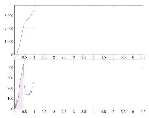
Das die Daten keine geometrische Form wiedergeben, ist erstmal noch kein Problem, aber die Menge der Daten mit den Spitzen in der Kurve ist es schon. Wenn man das darstellen und füllen will, ist Handarbeit nötig. Wenn man im zweiten Plot nur jeden 5.Punkt (each nth point=5) zum Zeichnen verwendet, bleibt die Form im Wesentlichen erhalten:

\documentclass[a4paper]{scrreprt}   
\usepackage{pgfplots} 
\pgfplotsset{compat=1.12} 
\usepgfplotslibrary{fillbetween} 
\usetikzlibrary{intersections} 
\begin{document} 
\begin{tikzpicture}[ 
   /pgfplots/every axis/.style={% 
     scale only axis, 
     width=13cm, 
     height=5cm, 
     xmin=0,xmax=6.5,
     enlarge y limits=upper
   } 
] 
\begin{axis}[name=plot1]% 
   \addplot [ 
       color=blue, 
       solid, 
       name path=A 
     ] 
     coordinates{ 
        (0.105,0)(0.11,11.9866)(0.115,36.5101)(0.12,61.0337)(0.125,85.5572)(0.13,110.081)(0.135,134.604)(0.14,159.128)(0.145,183.651)(0.15,208.175)(0.155,232.699)(0.16,257.222)(0.165,281.746)(0.17,306.269)(0.175,330.793)(0.18,355.316)(0.185,379.84)(0.19,404.363)(0.195,428.887)(0.2,453.41)(0.205,477.934)(0.21,502.458)(0.215,526.981)(0.22,551.505)(0.225,578.131)(0.23,607.435)(0.235,636.738)(0.24,666.042)(0.245,696.76)(0.25,728.504)(0.255,760.247)(0.26,793.14)(0.265,827.438)(0.27,861.736)(0.275,896.937)(0.28,932.304)(0.285,968.339)(0.29,1005.11)(0.295,1042.42)(0.3,1080.64)(0.305,1117.72)(0.31,1153.02)(0.315,1190.07)(0.32,1228.33)(0.325,1264.4)(0.33,1300.55)(0.335,1337.72)(0.34,1374.54)(0.345,1410.95)(0.35,1446.55)(0.355,1482.46)(0.36,1517.96)(0.365,1553.25)(0.37,1590.69)(0.375,1627.34)(0.38,1663.95)(0.385,1699.71)(0.39,1735.48)(0.395,1775.15)(0.4,1807.98)(0.405,1846.59)(0.41,1882.08)(0.415,1917.06)(0.42,1952.82)(0.425,1988.96)(0.43,2025.58)(0.435,2062.54)(0.44,2097.04)(0.445,2119.99)(0.45,2146.21)(0.455,2176.05)(0.46,2206.23)(0.465,2230.24)(0.47,2259.44)(0.475,2293.36)(0.48,2316.92)(0.485,2336.81)(0.49,2355.91)(0.495,2372.29)(0.5,2387.95)(0.505,2403.57)(0.51,2420.72)(0.515,2437.1)(0.52,2449.78)(0.525,2463.59)(0.53,2479.73)(0.535,2492.51)(0.54,2500.45)(0.545,2514.95)(0.55,2529.2)(0.555,2540.38)(0.56,2553.65)(0.565,2562.66)(0.57,2576.77)(0.575,2591.08)(0.58,2603.04)(0.585,2609.16)(0.59,2624.04)(0.595,2632.52)(0.6,2640.17)(0.605,2647.8)(0.61,2660.75)(0.615,2666.2)(0.62,2672.61)(0.625,2681.08)(0.63,2696.63)(0.635,2706.69)(0.64,2711.1)(0.645,2724.42)(0.65,2727.27)(0.655,2739.73)(0.66,2747.84)(0.665,2758.71)(0.67,2767.54)(0.675,2771.36)(0.68,2784.22)(0.685,2787.88)(0.69,2803.46)(0.695,2810.3)(0.7,2820.55)(0.705,2831.45)(0.71,2836.88)(0.715,2843.89)(0.72,2857.14)(0.725,2863.18)(0.73,2870.81)(0.735,2881.16)(0.74,2891.57)(0.745,2900.63)(0.75,2906.19)(0.755,2916.5)(0.76,2926.98)(0.765,2933.99)(0.77,2947.57)(0.775,2959.87)(0.78,2962.3)(0.785,2977.67)(0.79,2984.14)(0.795,2990.67)(0.8,3000)(0.805,3005.6)(0.81,3021.76)(0.815,3025.65)(0.82,3044.38)(0.825,3053.44)(0.83,3060.93)(0.835,3076.92)(0.84,3077.22)(0.845,3084.83)(0.85,3093.73)(0.855,3106.17)(0.86,3118.77)(0.865,3137.91)(0.87,3141.36)(0.875,3148.97)(0.88,3162.16)(0.885,3167.83)(0.89,3188.85)(0.895,3202.37)(0.9,3208.56)(0.905,3217.16)(0.91,3226.71)(0.915,3240.86)(0.92,3258.13)(0.925,3269.75)(0.93,3284.17)(0.935,3299.14)(0.94,3305.79)(0.945,3320.09)(0.95,3333.33)(0.955,3350.25)(0.96,3372.39)(0.965,3382.85)(0.97,3406.38)(0.975,3405.87)(0.98,3426.23)(0.985,3438.4)(0.99,3454.52)(0.995,3468.21)(1,3481.2) 
     }; 
   \draw[red, dashed, thick,name path=B](axis cs:0,2000) -- (axis cs:1,2000); 
   \path[name intersections={of=A and B, by=C}]; 
\end{axis} 

\begin{axis}[% 
   at=(plot1.below south west), anchor=above north west, 
]% 
   \addplot [ 
       color=blue, 
       solid, 
       name path=A,
       each nth point=5
     ] 
     coordinates{ 
        (0,-4.02538)(0.005,-3.01978)(0.01,-4.02525)(0.015,-4.0255)(0.02,-3.01959)(0.025,-3.01903)(0.03,-4.026)(0.035,-2.01288)(0.04,15.0825)(0.045,15.0778)(0.05,14.0761)(0.055,14.0761)(0.06,17.0935)(0.065,72.8791)(0.07,135.93)(0.075,125.77)(0.08,14.0615)(0.085,27.6092)(0.09,27.124)(0.095,32.106)(0.1,33.132)(0.105,36.6323)(0.11,38.1223)(0.115,43.1478)(0.12,43.1384)(0.125,49.1344)(0.13,51.5966)(0.135,58.0689)(0.14,60.06)(0.145,63.0453)(0.15,72.0045)(0.155,73.5689)(0.16,79.037)(0.165,85.0213)(0.17,88.8984)(0.175,90.3959)(0.18,105.858)(0.185,107.895)(0.19,117.687)(0.195,125.202)(0.2,120.187)(0.205,138.741)(0.21,148.851)(0.215,148.799)(0.22,152.056)(0.225,175.402)(0.23,190.966)(0.235,190.345)(0.24,192.956)(0.245,211.432)(0.25,225.9)(0.255,234.983)(0.26,252.8)(0.265,247.58)(0.27,249.83)(0.275,254.329)(0.28,272.239)(0.285,267.741)(0.29,269.179)(0.295,266.67)(0.3,288.294)(0.305,297.525)(0.31,292.202)(0.315,293.22)(0.32,306.813)(0.325,302.884)(0.33,302.295)(0.335,314.643)(0.34,314.626)(0.345,315.56)(0.35,332.803)(0.355,340.06)(0.36,343.391)(0.365,356.402)(0.37,345.998)(0.375,357.106)(0.38,352.769)(0.385,373.187)(0.39,370.35)(0.395,368.587)(0.4,392.196)(0.405,383.449)(0.41,380.49)(0.415,401.796)(0.42,398.224)(0.425,415.457)(0.43,409.486)(0.435,421.172)(0.44,417.584)(0.445,420.823)(0.45,431.708)(0.455,427.179)(0.46,365.727)(0.465,264.148)(0.47,262.717)(0.475,250.8)(0.48,252.038)(0.485,238.01)(0.49,238.043)(0.495,226.71)(0.5,215.738)(0.505,208.6)(0.51,208.987)(0.515,197.018)(0.52,191.154)(0.525,182.58)(0.53,178.178)(0.535,172.937)(0.54,174.554)(0.545,167.958)(0.55,162.176)(0.555,165.695)(0.56,159.281)(0.565,152.8)(0.57,154.698)(0.575,161.276)(0.58,148.814)(0.585,149.063)(0.59,142.553)(0.595,137.176)(0.6,138.114)(0.605,145.215)(0.61,135.724)(0.615,137.695)(0.62,139.055)(0.625,141.073)(0.63,130.312)(0.635,137.734)(0.64,137.189)(0.645,136.662)(0.65,130.247)(0.655,136.041)(0.66,136.302)(0.665,137.513)(0.67,130.809)(0.675,140.673)(0.68,138.742)(0.685,136.142)(0.69,136.242)(0.695,134.186)(0.7,136.384)(0.705,144.65)(0.71,134.655)(0.715,149.484)(0.72,145.092)(0.725,137.651)(0.73,141.135)(0.735,149.156)(0.74,144.067)(0.745,153.678)(0.75,151.007)(0.755,158.95)(0.76,153.857)(0.765,154.903)(0.77,144.554)(0.775,124.477)(0.78,125.378)(0.785,149.006)(0.79,152.015)(0.795,156.845)(0.8,165.789)(0.805,156.752)(0.81,167.453)(0.815,176.793)(0.82,173.655)(0.825,178.183)(0.83,175.656)(0.835,171.697)(0.84,171.411)(0.845,166.666)(0.85,155.96)(0.855,130.288)(0.86,144.076)(0.865,167.495)(0.87,171.286)(0.875,182.187)(0.88,195.055)(0.885,207.802)(0.89,210.589)(0.895,197.18)(0.9,222.632)(0.905,211.144)(0.91,202.026)(0.915,177.845)(0.92,204.964)(0.925,224.333)(0.93,220.948)(0.935,228.89)(0.94,233.336)(0.945,240.538)(0.95,250.69)(0.955,253.347)(0.96,237.966)(0.965,245.889)(0.97,251.459)(0.975,256.437)(0.98,253.75)(0.985,266.188)(0.99,259.732)(0.995,267.656)(1,261.237) 
     }; 
   \path [name path=B] 
    (\pgfkeysvalueof{/pgfplots/xmin},{\pgfkeysvalueof{/pgfplots/ymin}})--(\pgfkeysvalueof{/pgfplots/xmax},\pgfkeysvalueof{/pgfplots/ymin}); 
   \addplot[purple!10]fill between[ 
     of= A and B, every odd segment/.style={green},
    soft clip={(0,\pgfkeysvalueof{/pgfplots/ymin})rectangle(C|-current axis.north)}
     ]; 
\end{axis} 
\draw[dashed,thin](C)--(C|-current axis.south); 
\end{tikzpicture} 
\end{document}

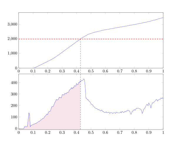
In dem Beispiel habe ich auch der Pfad B im zweiten Plot und der soft Clip path etwas geändert.

Bild

Statt nur jeden 5.Punkt zu verwenden, wäre es vermutlich besser xmax anzupassen. Allerdings muss dabei aus irgendeinem Grund enlarge y limits=upper durch ymin=-10 mit einem ausreichend großen (bezogen auf den Betrag) negativen Wert verwendet werden, warum auch immer.

Bild

\documentclass[a4paper]{scrreprt}   
\usepackage{pgfplots} 
\pgfplotsset{compat=1.12} 
\usepgfplotslibrary{fillbetween} 
\usetikzlibrary{intersections} 
\begin{document} 
\begin{tikzpicture}[ 
   /pgfplots/every axis/.style={% 
     scale only axis, 
     width=13cm, 
     height=5cm, 
     xmin=0,xmax=1,
     ymin=-10
   } 
] 
\begin{axis}[name=plot1]% 
   \addplot [ 
       color=blue, 
       solid, 
       name path=A 
     ] 
     coordinates{ 
        (0.105,0)(0.11,11.9866)(0.115,36.5101)(0.12,61.0337)(0.125,85.5572)(0.13,110.081)(0.135,134.604)(0.14,159.128)(0.145,183.651)(0.15,208.175)(0.155,232.699)(0.16,257.222)(0.165,281.746)(0.17,306.269)(0.175,330.793)(0.18,355.316)(0.185,379.84)(0.19,404.363)(0.195,428.887)(0.2,453.41)(0.205,477.934)(0.21,502.458)(0.215,526.981)(0.22,551.505)(0.225,578.131)(0.23,607.435)(0.235,636.738)(0.24,666.042)(0.245,696.76)(0.25,728.504)(0.255,760.247)(0.26,793.14)(0.265,827.438)(0.27,861.736)(0.275,896.937)(0.28,932.304)(0.285,968.339)(0.29,1005.11)(0.295,1042.42)(0.3,1080.64)(0.305,1117.72)(0.31,1153.02)(0.315,1190.07)(0.32,1228.33)(0.325,1264.4)(0.33,1300.55)(0.335,1337.72)(0.34,1374.54)(0.345,1410.95)(0.35,1446.55)(0.355,1482.46)(0.36,1517.96)(0.365,1553.25)(0.37,1590.69)(0.375,1627.34)(0.38,1663.95)(0.385,1699.71)(0.39,1735.48)(0.395,1775.15)(0.4,1807.98)(0.405,1846.59)(0.41,1882.08)(0.415,1917.06)(0.42,1952.82)(0.425,1988.96)(0.43,2025.58)(0.435,2062.54)(0.44,2097.04)(0.445,2119.99)(0.45,2146.21)(0.455,2176.05)(0.46,2206.23)(0.465,2230.24)(0.47,2259.44)(0.475,2293.36)(0.48,2316.92)(0.485,2336.81)(0.49,2355.91)(0.495,2372.29)(0.5,2387.95)(0.505,2403.57)(0.51,2420.72)(0.515,2437.1)(0.52,2449.78)(0.525,2463.59)(0.53,2479.73)(0.535,2492.51)(0.54,2500.45)(0.545,2514.95)(0.55,2529.2)(0.555,2540.38)(0.56,2553.65)(0.565,2562.66)(0.57,2576.77)(0.575,2591.08)(0.58,2603.04)(0.585,2609.16)(0.59,2624.04)(0.595,2632.52)(0.6,2640.17)(0.605,2647.8)(0.61,2660.75)(0.615,2666.2)(0.62,2672.61)(0.625,2681.08)(0.63,2696.63)(0.635,2706.69)(0.64,2711.1)(0.645,2724.42)(0.65,2727.27)(0.655,2739.73)(0.66,2747.84)(0.665,2758.71)(0.67,2767.54)(0.675,2771.36)(0.68,2784.22)(0.685,2787.88)(0.69,2803.46)(0.695,2810.3)(0.7,2820.55)(0.705,2831.45)(0.71,2836.88)(0.715,2843.89)(0.72,2857.14)(0.725,2863.18)(0.73,2870.81)(0.735,2881.16)(0.74,2891.57)(0.745,2900.63)(0.75,2906.19)(0.755,2916.5)(0.76,2926.98)(0.765,2933.99)(0.77,2947.57)(0.775,2959.87)(0.78,2962.3)(0.785,2977.67)(0.79,2984.14)(0.795,2990.67)(0.8,3000)(0.805,3005.6)(0.81,3021.76)(0.815,3025.65)(0.82,3044.38)(0.825,3053.44)(0.83,3060.93)(0.835,3076.92)(0.84,3077.22)(0.845,3084.83)(0.85,3093.73)(0.855,3106.17)(0.86,3118.77)(0.865,3137.91)(0.87,3141.36)(0.875,3148.97)(0.88,3162.16)(0.885,3167.83)(0.89,3188.85)(0.895,3202.37)(0.9,3208.56)(0.905,3217.16)(0.91,3226.71)(0.915,3240.86)(0.92,3258.13)(0.925,3269.75)(0.93,3284.17)(0.935,3299.14)(0.94,3305.79)(0.945,3320.09)(0.95,3333.33)(0.955,3350.25)(0.96,3372.39)(0.965,3382.85)(0.97,3406.38)(0.975,3405.87)(0.98,3426.23)(0.985,3438.4)(0.99,3454.52)(0.995,3468.21)(1,3481.2) 
     }; 
   \draw[red, dashed, thick,name path=B](axis cs:0,2000) -- (axis cs:1,2000); 
   \path[name intersections={of=A and B, by=C}]; 
\end{axis} 

\begin{axis}[% 
   at=(plot1.below south west), anchor=above north west, 
]% 
   \addplot [ 
       color=blue, 
       solid, 
       name path=A,
       each nth point=1
     ] 
     coordinates{ 
        (0,-4.02538)(0.005,-3.01978)(0.01,-4.02525)(0.015,-4.0255)(0.02,-3.01959)(0.025,-3.01903)(0.03,-4.026)(0.035,-2.01288)(0.04,15.0825)(0.045,15.0778)(0.05,14.0761)(0.055,14.0761)(0.06,17.0935)(0.065,72.8791)(0.07,135.93)(0.075,125.77)(0.08,14.0615)(0.085,27.6092)(0.09,27.124)(0.095,32.106)(0.1,33.132)(0.105,36.6323)(0.11,38.1223)(0.115,43.1478)(0.12,43.1384)(0.125,49.1344)(0.13,51.5966)(0.135,58.0689)(0.14,60.06)(0.145,63.0453)(0.15,72.0045)(0.155,73.5689)(0.16,79.037)(0.165,85.0213)(0.17,88.8984)(0.175,90.3959)(0.18,105.858)(0.185,107.895)(0.19,117.687)(0.195,125.202)(0.2,120.187)(0.205,138.741)(0.21,148.851)(0.215,148.799)(0.22,152.056)(0.225,175.402)(0.23,190.966)(0.235,190.345)(0.24,192.956)(0.245,211.432)(0.25,225.9)(0.255,234.983)(0.26,252.8)(0.265,247.58)(0.27,249.83)(0.275,254.329)(0.28,272.239)(0.285,267.741)(0.29,269.179)(0.295,266.67)(0.3,288.294)(0.305,297.525)(0.31,292.202)(0.315,293.22)(0.32,306.813)(0.325,302.884)(0.33,302.295)(0.335,314.643)(0.34,314.626)(0.345,315.56)(0.35,332.803)(0.355,340.06)(0.36,343.391)(0.365,356.402)(0.37,345.998)(0.375,357.106)(0.38,352.769)(0.385,373.187)(0.39,370.35)(0.395,368.587)(0.4,392.196)(0.405,383.449)(0.41,380.49)(0.415,401.796)(0.42,398.224)(0.425,415.457)(0.43,409.486)(0.435,421.172)(0.44,417.584)(0.445,420.823)(0.45,431.708)(0.455,427.179)(0.46,365.727)(0.465,264.148)(0.47,262.717)(0.475,250.8)(0.48,252.038)(0.485,238.01)(0.49,238.043)(0.495,226.71)(0.5,215.738)(0.505,208.6)(0.51,208.987)(0.515,197.018)(0.52,191.154)(0.525,182.58)(0.53,178.178)(0.535,172.937)(0.54,174.554)(0.545,167.958)(0.55,162.176)(0.555,165.695)(0.56,159.281)(0.565,152.8)(0.57,154.698)(0.575,161.276)(0.58,148.814)(0.585,149.063)(0.59,142.553)(0.595,137.176)(0.6,138.114)(0.605,145.215)(0.61,135.724)(0.615,137.695)(0.62,139.055)(0.625,141.073)(0.63,130.312)(0.635,137.734)(0.64,137.189)(0.645,136.662)(0.65,130.247)(0.655,136.041)(0.66,136.302)(0.665,137.513)(0.67,130.809)(0.675,140.673)(0.68,138.742)(0.685,136.142)(0.69,136.242)(0.695,134.186)(0.7,136.384)(0.705,144.65)(0.71,134.655)(0.715,149.484)(0.72,145.092)(0.725,137.651)(0.73,141.135)(0.735,149.156)(0.74,144.067)(0.745,153.678)(0.75,151.007)(0.755,158.95)(0.76,153.857)(0.765,154.903)(0.77,144.554)(0.775,124.477)(0.78,125.378)(0.785,149.006)(0.79,152.015)(0.795,156.845)(0.8,165.789)(0.805,156.752)(0.81,167.453)(0.815,176.793)(0.82,173.655)(0.825,178.183)(0.83,175.656)(0.835,171.697)(0.84,171.411)(0.845,166.666)(0.85,155.96)(0.855,130.288)(0.86,144.076)(0.865,167.495)(0.87,171.286)(0.875,182.187)(0.88,195.055)(0.885,207.802)(0.89,210.589)(0.895,197.18)(0.9,222.632)(0.905,211.144)(0.91,202.026)(0.915,177.845)(0.92,204.964)(0.925,224.333)(0.93,220.948)(0.935,228.89)(0.94,233.336)(0.945,240.538)(0.95,250.69)(0.955,253.347)(0.96,237.966)(0.965,245.889)(0.97,251.459)(0.975,256.437)(0.98,253.75)(0.985,266.188)(0.99,259.732)(0.995,267.656)(1,261.237) 
     }; 
   \path [name path=B] 
    (\pgfkeysvalueof{/pgfplots/xmin},{\pgfkeysvalueof{/pgfplots/ymin}})--(\pgfkeysvalueof{/pgfplots/xmax},\pgfkeysvalueof{/pgfplots/ymin}); 
   \addplot[purple!10]fill between[ 
     of= A and B, every odd segment/.style={green},
     soft clip={(0,\pgfkeysvalueof{/pgfplots/ymin})rectangle(C|-current axis.north)}
     ]; 
\end{axis} 
\draw[dashed,thin](C)--(C|-current axis.south); 
\end{tikzpicture} 
\end{document}

Gruß
Elke