LaTeX Forum

von **feuerfalke2005** » Di 31. Mai 2016, 09:59

Danke für die Hilfe
Und für die Hinweise das ich besser auf passe das die Beispiel auch lauffähig sind.

Könntest Du mir bitte noch angeben wie man die Pins der Bezeichnungen eventuell von der Lage her einstellen kann?
Also recht oder licks bzw mitte.
Und kann man da auch eine Legende der Farben irgend wie eintragen?

Noch mals vielen Danke hat mir wirklich gut geholfen.

von **esdd** » Di 31. Mai 2016, 09:06

Bitte erstelle immer lauffähige Beispiele. Oben fehlen sowohl \begin{document} als auch \end{document} und die Datei fürs Plotten wird so auch nicht bei anderen gefunden.

Wie Einheiten richtig angegeben werden, hat Dir Bartmann eigentlich in dem anderen Thread schon mal gezeigt. Ich korrigiere das jetzt nicht nochmal.

\begin{filecontents*}{NS2.dat} 
 0 33.525 
 125 84.85 
 375 187.5 
\end{filecontents*} 

\documentclass[11pt]{article} 
\usepackage[T1]{fontenc} 
\usepackage[utf8]{inputenc} 
\usepackage{pgfplots} 
\pgfplotsset{compat=1.13} 
\usetikzlibrary{decorations.pathreplacing}
\begin{document}
\begin{figure}[htb] 
    \begin{tikzpicture}[pin edge={thick,<-,shorten <=2pt,black},pin distance=5ex,every pin/.style={draw,text=black}],decoration=brase] 
    \begin{axis}[ 
    width=12cm, 
    height=8cm, 
    scale only axis, 
    xmin=0, 
    xmax=400, 
    xtick={0,25,...,400}, 
    xlabel={Normalspannung $\sigma$ in [$\frac{kN}{m^2}$]}, 
    ymin=0, 
    ymax=200, 
    ylabel={Scherspannung $\tau$ $\frac{kN}{m^2}$}, 
    axis x line*=bottom, %top, 
    axis y line*=left, 
    grid=major, 
    every axis plot/.append style={ 
       line width=1.5pt, 
       mark size=2pt, 
       mark=ball, 
       forget plot, 
       visualization depends on={x \as \xvalue}, 
    }, 
    point meta=y, 
    nodes near coords={}, 
    nodes near coords style={ 
       inner sep=0pt, 
       pin=left:{\pgfmathprintnumber{\xvalue}, \pgfmathprintnumber{\pgfplotspointmeta}} 
    }, 
    ] 
    \addplot[red] coordinates {(0,33.53)} 
    coordinate(h)--(h|-0,0) 
    ; 
    \addplot[red] coordinates {(125,84.85)} 
    coordinate(h)--(h|-0,0) 
    ; 
    \addplot[green] coordinates {(250,148.22)} 
    coordinate(h)--(h|-0,0) 
    ; 
    \addplot[blue]coordinates{(375,187.5)} 
    coordinate(h)--(h|-0,0) 
    ; 
    \addplot [black,no markers,every node near coord/.style={}] 
    table {NS2.dat}coordinate[pos=0](s);
    \draw[decorate,decoration={brace,amplitude=5pt},very thick] 
      (s) 
      -- node[blue,anchor=west,align=left,inner sep=10pt,font=\small] {Scheinbare Kohäsion\\33,53 $\frac{kN}{m^2}$}
      (0,0);
    \end{axis} 
    
\end{tikzpicture} 
    \caption{Normal-Scherspannungs - Diagramm} 
    \label{Normalspannung}
\end{figure}
\end{document}

von **feuerfalke2005** » Di 31. Mai 2016, 08:13

Danke esdd

Das habe ich mal komplett übernommen und Funktioniert tadel los, und noch ein paar kleinigkeiten ergänz die in meiner erklärung wohl untergegangen waren danke nochmals.
Ich gebe mal deinen Quelltext mit meinen anpassungen hier ein.

Ich hätte da noch eine Frage wie bekomme ich eine dicke Geschweifte Klammer in der nähe der y Achse Gezeichnet ich hatte das soweit hin bekommen aber das waren auf einmal 3 stück. Ist in der draw Zeile am Ende eingetragen. Leider macht es nun nur noch den Text aber nicht mehr die Geschweifte klammer.

\begin{filecontents*}{NS2.dat}
0 33.525
125 84.85
375 187.5
\end{filecontents*}

\documentclass[11pt]{article}
\usepackage[T1]{fontenc}
\usepackage[utf8]{inputenc}
\usepackage{pgfplots}
\pgfplotsset{compat=1.13}

\begin{document}


\begin{figure}[H]
	\begin{tikzpicture}[pin edge={thick,<-,shorten <=2pt,black},pin distance=5ex,every pin/.style={draw,text=black}],decoration=brase]
	\begin{axis}[
	width=12cm,
	height=8cm,
	scale only axis,
	xmin=0,
	xmax=400,
	xtick={0,25,...,400},
	xlabel={Normalspannung $\sigma$ in [$\frac{kN}{m^2}$]},
	ymin=0,
	ymax=200,
	ylabel={Scherspannung $\tau$ $\frac{kN}{m^2}$},
	axis x line*=bottom, %top,
	axis y line*=left,
	grid=major,
	every axis plot/.append style={
		line width=1.5pt,
		mark size=2pt,
		mark=ball,
		forget plot,
		visualization depends on={x \as \xvalue},
	},
	point meta=y,
	nodes near coords={},
	nodes near coords style={
		inner sep=0pt,
		pin=left:{\pgfmathprintnumber{\xvalue}, \pgfmathprintnumber{\pgfplotspointmeta}}
	},
	]
	\addplot[red] coordinates {(0,33.53)}
	coordinate(h)--(h|-0,0)
	;
	\addplot[red] coordinates {(125,84.85)}
	coordinate(h)--(h|-0,0)
	;
	\addplot[green] coordinates {(250,148.22)}
	coordinate(h)--(h|-0,0)
	;
	\addplot[blue]coordinates{(375,187.5)}
	coordinate(h)--(h|-0,0)
	;
	\addplot [black,no markers,every node near coord/.style={}]
	table[restrict expr to domain={\thisrowno{0}}{0:375}] {NS2.dat};
	\end{axis}
	\draw[decorate, yshift=0ex] (0,1.65) -- node[blue,anchor=base west, xshift=2ex] {Scheinbare Koh\"asion 33,53 $\frac{kN}{m^2}$} (0,0);% Geschweifte Klammer mit schrift recht 
\end{tikzpicture}
	\caption{Normal-Scherspannungs - Diagramm}
	\label{Normalspannung}
\end{figure}
\end{document}

Darstellung des Oberen Quelltextes

Bild

Nochmals Danke für die Hilfe

von **esdd** » Di 31. Mai 2016, 01:30

Eine Möglichkeit wäre

\begin{filecontents*}{NS2.dat}
0 33.525
125 84.85
375 187.5
\end{filecontents*}

\documentclass[11pt]{article}
\usepackage[T1]{fontenc}
\usepackage[utf8]{inputenc}
\usepackage{pgfplots}
\pgfplotsset{compat=1.13}

\begin{document}
\begin{figure}
  \begin{tikzpicture}[pin edge={thick,<-,shorten <=2pt,black},pin distance=5ex,every pin/.style={draw,text=black}]
    \begin{axis}[
        width=14cm,
        height=10cm,
        scale only axis,
        xmin=0,
        xmax=400,
        xtick={0,25,...,400},
        xlabel={Normalspannung $\sigma$ in [$\frac{kN}{m^2}$]},
        ymin=0,
        ymax=200,
        ylabel={Scherspannung $\tau$ $\frac{kN}{m^2}$},
        axis x line*=bottom, %top,
        axis y line*=left,
        grid=major,
        every axis plot/.append style={
           line width=1.5pt,
           mark size=2pt,
           mark=ball,
           forget plot,
           visualization depends on={x \as \xvalue},
        },
        point meta=y,
        nodes near coords={},
        nodes near coords style={
          inner sep=0pt,
          pin=left:{\pgfmathprintnumber{\xvalue}, \pgfmathprintnumber{\pgfplotspointmeta}}
        },
    ]
   \addplot[red] coordinates {(125,84.85)}
     coordinate(h)--(h|-0,0)
   ;
   \addplot[green] coordinates {(250,148.22)}
     coordinate(h)--(h|-0,0)
   ;
   \addplot[blue]coordinates{(375,187.5)}
     coordinate(h)--(h|-0,0)
   ;
   \addplot [black,no markers,every node near coord/.style={}] 
      table[restrict expr to domain={\thisrowno{0}}{125:375}] {NS2.dat};
   \end{axis}
  \end{tikzpicture}
  \caption{Normal-Scherspannungs - Diagramm}
\end{figure}
\end{document}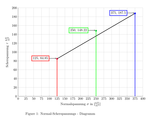

Falls ein Teil der Beschriftungen außerhalb des Plotbereichs liegt, muss in dem Fall die Option clip=false ergänzt werden.

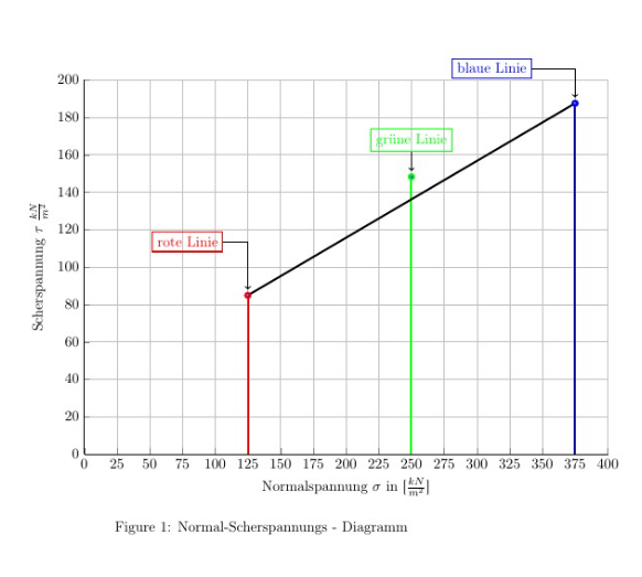
Andere Möglichkeit:

\begin{filecontents*}{NS2.dat}
0 33.525
125 84.85
375 187.5
\end{filecontents*}

\documentclass[11pt]{article}
\usepackage[T1]{fontenc}
\usepackage[utf8]{inputenc}
\usepackage{pgfplots}
\pgfplotsset{compat=1.12}% aktuell ist 1.13, aber Overleaf hat nur 1.12
\usetikzlibrary{positioning}
\begin{document}
\begin{figure}
  \begin{tikzpicture}
    \begin{axis}[
        width=14cm,
        height=10cm,
        scale only axis,
        xmin=0,
        xmax=400,
        xtick={0,25,...,400},
        xlabel={Normalspannung $\sigma$ in [$\frac{kN}{m^2}$]},
        ymin=0,
        ymax=200,
        ylabel={Scherspannung $\tau$ $\frac{kN}{m^2}$},
        axis x line*=bottom, %top,
        axis y line*=left,
        grid=major,
        every axis plot/.append style={
           line width=1.5pt,
           mark size=2pt,
           mark=ball,
           forget plot,
        },
    ]
   \addplot[red] coordinates {(125,84.85)}
     node(h1){}--(h1|-0,0)
   ;
   \addplot[green] coordinates {(250,148.22)}
     node(h2){}--(h2|-0,0)
   ;
   \addplot[blue]coordinates{(375,187.5)}
     node(h3){}--(h3|-0,0)
   ;
   \addplot [black,no markers,every node near coord/.style={}] 
      table[restrict expr to domain={\thisrowno{0}}{125:375}] {NS2.dat};
   \end{axis}
   \begin{scope}[nodes=draw,thick,->]
     \node[red,above left= 1cm and .5cm of h1](l1) {rote Linie};
     \draw (l1)-|(h1);
     \node[green,above=.5cm of h2](l2){grüne Linie};
     \draw (l2)--(h2);
     \node[blue,above left=.5cm and 1cm of h3](l3) {blaue Linie};
     \draw (l3)-|(h3);
   \end{scope}
  \end{tikzpicture}
  \caption{Normal-Scherspannungs - Diagramm}
\end{figure}
\end{document}

von **Bartman** » Mo 30. Mai 2016, 19:32

feuerfalke2005 hat geschrieben:Könntet Ihr mir hier weiter helfen wie ich es hin bekomme das die werte der x Achse in 25 Schritten erstellt werden

Füge

xtick={0,25,...,400},

der Liste der optionalen Argumente Deiner axis-Umgebung hinzu.

Da Deine beiden Textdateien im Anhang nicht mehr benötigt werden, darfst Du sie über den "Datei löschen"-Button entfernen.

von **feuerfalke2005** » Mo 30. Mai 2016, 16:10

Danke für die Hinweise

von **Bartman** » Mo 30. Mai 2016, 16:07

Setze Deine beiden filecontents-Umgebungen nach [code] und vor den Befehl \documentclass.

Bitte entferne auch die zwei Zeilen mit [code][/code] nach Deiner Danksagung.

von **feuerfalke2005** » Mo 30. Mai 2016, 15:40

Danke für die Hinweise
hoffe habe jetzt alle sorichtig eingestellt wie es erforderlich ist.

Danke für die Unterstützung

von **Bartman** » Mo 30. Mai 2016, 14:30

Benutze bitte für die Daten aus Deinen angehängten Dateien NS.dat und NS2.dat jeweils eine filecontents-Umgebung, wie es Dir esdd in Deinem anderen Thread vorgeführt hat. So hat man alles im Blick und muss nicht herumklicken.

Ersetze

[img]
http://golatex.de/files/normalspannung_101.png
[/img]

durch

[img]http://golatex.de/files/normalspannung_101.png[/img]

von **feuerfalke2005** » Mo 30. Mai 2016, 13:42

Hallo Liebe Latex Gemeinde
Ich schreibe hier meinen 2 Beitrag bzw. Frage
ich habe aus der Hilfe die mir in meiner 1 Frage gegeben wurde diesen Quelltext entwickelt.
gibt es hier noch andere möglichkeiten für Koordinaten zu diesen Anfang
nodes near coords={

Ich würde gerne Textboxen mit sogenanten fahnen verwenden
könnte mir jemand mitteilen wie man das macht.
Danke

Bild

\begin{filecontents*}{NS.dat}
    125 0
125 84.85
250 0
250 148.22
375 0
375 187.5 
\end{filecontents*}

\begin{filecontents*}{NS2.dat}
     0 33.525
125 84.85
375 187.5 
\end{filecontents*}


\documentclass[11pt]{article}
\usepackage[T1]{fontenc}
\usepackage{pgfplots}

\pgfplotsset{compat=1.12}  % Wenn nötig, Versionsnummer runter oder auf »newest« setzen

\begin{document}

\begin{figure}
  \begin{tikzpicture}
  \begin{axis}[
  width=14cm,
  height=10cm,
  scale only axis,
  xmin=0,
  xmax=400,
  xlabel={Normalspannung $\sigma$ in [$\frac{kN}{m^2}$]},
  ymin=0,
  ymax=200,
  ylabel={Scherspannung $\tau$ $\frac{kN}{m^2}$},
  axis x line*=bottom, %top,
  axis y line*=left,
  grid=major,
  every axis plot/.append style={
  	line width=1.5pt,
  	mark size=2pt,
  	mark=ball,forget plot,
  	visualization depends on={x \as \myvalue},
  },
  point meta=y,    
  nodes near coords={ 
  	\ifdim \myvalue pt=125pt \pgfmathprintnumber{\pgfplotspointmeta}\fi
  	\ifdim \myvalue pt=250pt \pgfmathprintnumber{\pgfplotspointmeta}\fi
  	\ifdim \myvalue pt=375pt \pgfmathprintnumber{\pgfplotspointmeta}\fi
  },
  nodes near coords style={text=black}
  ]
 \addplot [red] table[restrict expr to domain={\thisrowno{0}}{0:125}] {NS.dat};
 \addplot [green] table[restrict expr to domain={\thisrowno{0}}{250:250}] {NS.dat};
 \addplot [blue] table[restrict expr to domain={\thisrowno{0}}{375:375}] {NS.dat};
 \addplot [black] table[restrict expr to domain={\thisrowno{0}}{125:375}] {NS2.dat};
% \addplot [orange] table[restrict expr to domain={\thisrowno{0}}{0:375}] {datenNS.dat};
  \end{axis}
  \end{tikzpicture}
	\caption{Normal-Scherspannungs - Diagramm}
\end{figure}

\end{document}

Könntet Ihr mir hier weiter helfen wie ich es hin bekomme das die werte der x Achse in 25 Schritten erstellt werden und auf der Y Achse die Schwarze Linie zwischen den Punkten 84.85 und 187.5 einen schnittpunkt bildet
Ebenso intressant wäre es zu wissen wie man die Markierungen Mark=ball für die einzelnen Linien/Graphen steuer kann.

Kann mir noch jemand helfen zu verstehen wie die Syntax von Pgfplots über haupt zu verstehen bzw anzu wenden ist.

Danke für die Hilfe

LaTeX Forum

Graphendarstellung mit verschiedenen Farben

Antwort erstellen

Ansicht erweitern Die letzten Beiträge des Themas: Graphendarstellung mit verschiedenen Farben

Graphendarstellung mit verschiedenen Farben