von Krachi » Mi 1. Aug 2018, 09:56
Hi,
folgenden Code für eine tikz-Zeichnung habe ich geschrieben:
\documentclass{standalone}
\usepackage{pgfplots}
%\usepackage{../myMacros}
\usepackage{lmodern,textcomp}
\usepackage{amsmath}
\usetikzlibrary{arrows.meta}

\begin{document}

\pgfmathdeclarefunction{gauss}{3}{%
  \pgfmathparse{1/(#3*sqrt(2*pi))*exp(-((#1-#2)^2)/(2*#3^2))}%
}

\pgfmathdeclarefunction{linear}{1}{%
  \pgfmathparse{0.25*#1}%
}

\pgfmathdeclarefunction{tanhh}{1}{%
  \pgfmathparse{(tanh(#1*0.5-2)+1)*0.8}%
}

\begin{tikzpicture}

  \begin{axis}[ ymin=0,ymax=2,
								xmin=0,xmax=10,
								height=6cm,
								width=8cm,scale only axis,
								xticklabel=\empty,yticklabel=\empty,
								xtick=\empty,ytick=\empty,
                axis lines = middle,
							  xlabel=$x$,ylabel=$y$,
								label style = {at={(ticklabel cs:1.1)}},
								no markers,
								xshift=0,
								samples=200,
								domain=0:10]


  \addplot[ultra thick,restrict x to domain=2:8] {gauss(x, 5, 1)}
	coordinate [pos=0.35] (r1)
  coordinate [pos=0.65] (r2)
  coordinate [pos=0.5] (rm);

 \addplot[ultra thick,restrict x to domain=0:8] {linear(x)};
 \addplot[ultra thick,restrict x to domain=2:8] {linear(x)}
	coordinate [pos=0.35] (l1)
  coordinate [pos=0.65] (l2)
  coordinate [pos=0.5] (lm)
	coordinate (P1) at (axis description cs:0.5,0.5)
	;

 \end{axis}

	\pgfmathsetmacro\valueA{gauss(0, 3, 1)}

	\begin{axis}[
  clip=false,
  samples=200,
  ymin=0,ymax=2,
  xmin=0,xmax=10,
	height=6cm,
	width=8cm,scale only axis,
  rotate=90,
  domain=0:10,
	xshift=7.75cm,
  %at={(axis1.south west)},
  hide axis,
  anchor=south east,
]

\addplot[ultra thick,restrict x to domain=2.5:7.5,rotate=180] {gauss(x, 5, 0.8)}
  coordinate [pos=.325] (g1)
  coordinate [pos=0.675] (g2)
  coordinate [pos=0.5] (gm)
	coordinate (P2) at (axis description cs:1,0.5);

\end{axis}

%\draw [dashed] (r1) -- (l1);
%\draw [dashed] (r2) -- (l2);
%\draw [dashed] (rm) -- (lm);

\draw [dotted] (r1) |- (g2);
\draw [dotted] (r2) |- (g1);
\draw [dotted] (rm) |- (gm);

%\draw (P1) -| (P2);
%\draw (P1) circle (10pt);
%\draw (P2) circle (10pt);

\end{tikzpicture}

\begin{tikzpicture}

  \begin{axis}[ ymin=0,ymax=2,
								xmin=0,xmax=10,
								height=6cm,
								width=8cm,scale only axis,
								xticklabel=\empty,yticklabel=\empty,
								xtick=\empty,ytick=\empty,
                axis lines = middle,
							  xlabel=$x$,ylabel=$y$,
								label style = {at={(ticklabel cs:1.1)}},
								no markers,
								xshift=0,
								samples=200,
								domain=0:10]


  \addplot[ultra thick,restrict x to domain=2:8] {gauss(x, 5, 1)}
	coordinate [pos=0.35] (r1)
  coordinate [pos=0.65] (r2)
  coordinate [pos=0.5] (rm);

 \addplot[ultra thick,restrict x to domain=0:8] {tanhh(x)};
 \addplot[ultra thick,restrict x to domain=2:8] {tanhh(x)}
	coordinate [pos=0.35] (l1)
  coordinate [pos=0.65] (l2)
  coordinate [pos=0.5] (lm);
	coordinate (P1) at (axis description cs:0.5,0.5)
	;

 \end{axis}

	\begin{axis}[
  clip=false,
  samples=200,
  ymin=0,ymax=2,
  xmin=0,xmax=10,
	height=6cm,
	width=8cm,scale only axis,
  rotate=90,
  domain=0:10,
	xshift=7.75cm,
  %at={(axis1.south west)},
  hide axis,
  anchor=south east,
]

\addplot[ultra thick,restrict x to domain=2.5:7.5,rotate=180] {gauss(x, 5, 0.8)}
  coordinate [pos=.325] (g1)
  coordinate [pos=0.675] (g2)
  coordinate [pos=0.5] (gm)
	coordinate (P2) at (axis description cs:1,0.5);

\end{axis}

\draw [dashed] (r1) -- (l1);
\draw [dashed] (r2) -- (l2);
\draw [dashed] (rm) -- (lm);

%\draw [dotted] (r1) |- (g2);
%\draw [dotted] (r2) |- (g1);
%\draw [dotted] (rm) |- (gm);

%\draw (P1) -| (P2);
%\draw (P1) circle (10pt);
%\draw (P2) circle (10pt);

\end{tikzpicture}

\end{document}
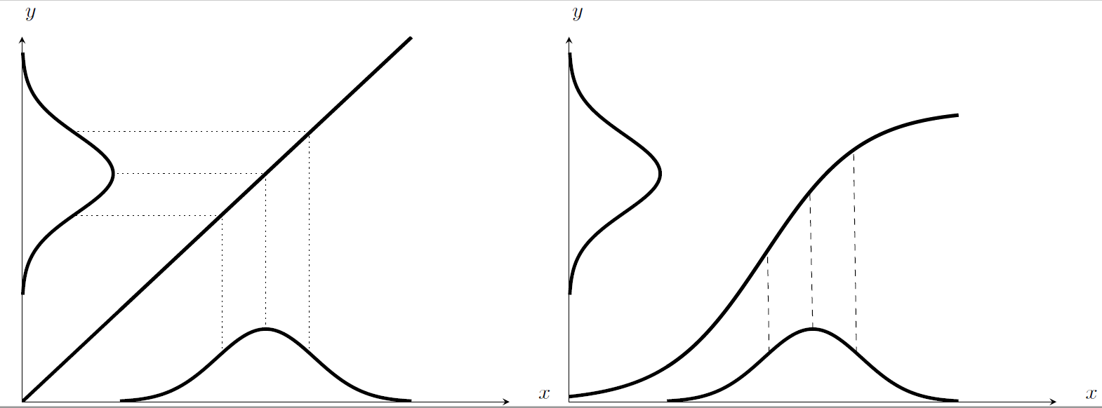
Dabei möchte ich, dass auch in der rechten Abbildung die Linien, ausgehend von der Gaußkurve senkrecht nach oben gehen, an den jeweiligen Stellen der nichtlinearen Funktion abknicken und dann waagerecht weiter auf die andere Gaußkurve abbilden (wie in der linken Abbildung).
Könnte mir jemand erklären, wie ich das machen könnte? Die Linien sind bisher schief, was wohl daran liegt, dass ich relativ für jeden Plot Koordinaten bilde und nicht explizit Koordinaten an den Stellen der Funktionen ausrechne. Leider hab ich das bisher nicht lösen können...
Gruß,
Max
- Dateianhänge
-
- Zeichnung.png (28.63 KiB) 2012 mal betrachtet
Hi,
folgenden Code für eine tikz-Zeichnung habe ich geschrieben:
[code]
\documentclass{standalone}
\usepackage{pgfplots}
%\usepackage{../myMacros}
\usepackage{lmodern,textcomp}
\usepackage{amsmath}
\usetikzlibrary{arrows.meta}
\begin{document}
\pgfmathdeclarefunction{gauss}{3}{%
\pgfmathparse{1/(#3*sqrt(2*pi))*exp(-((#1-#2)^2)/(2*#3^2))}%
}
\pgfmathdeclarefunction{linear}{1}{%
\pgfmathparse{0.25*#1}%
}
\pgfmathdeclarefunction{tanhh}{1}{%
\pgfmathparse{(tanh(#1*0.5-2)+1)*0.8}%
}
\begin{tikzpicture}
\begin{axis}[ ymin=0,ymax=2,
xmin=0,xmax=10,
height=6cm,
width=8cm,scale only axis,
xticklabel=\empty,yticklabel=\empty,
xtick=\empty,ytick=\empty,
axis lines = middle,
xlabel=$x$,ylabel=$y$,
label style = {at={(ticklabel cs:1.1)}},
no markers,
xshift=0,
samples=200,
domain=0:10]
\addplot[ultra thick,restrict x to domain=2:8] {gauss(x, 5, 1)}
coordinate [pos=0.35] (r1)
coordinate [pos=0.65] (r2)
coordinate [pos=0.5] (rm);
\addplot[ultra thick,restrict x to domain=0:8] {linear(x)};
\addplot[ultra thick,restrict x to domain=2:8] {linear(x)}
coordinate [pos=0.35] (l1)
coordinate [pos=0.65] (l2)
coordinate [pos=0.5] (lm)
coordinate (P1) at (axis description cs:0.5,0.5)
;
\end{axis}
\pgfmathsetmacro\valueA{gauss(0, 3, 1)}
\begin{axis}[
clip=false,
samples=200,
ymin=0,ymax=2,
xmin=0,xmax=10,
height=6cm,
width=8cm,scale only axis,
rotate=90,
domain=0:10,
xshift=7.75cm,
%at={(axis1.south west)},
hide axis,
anchor=south east,
]
\addplot[ultra thick,restrict x to domain=2.5:7.5,rotate=180] {gauss(x, 5, 0.8)}
coordinate [pos=.325] (g1)
coordinate [pos=0.675] (g2)
coordinate [pos=0.5] (gm)
coordinate (P2) at (axis description cs:1,0.5);
\end{axis}
%\draw [dashed] (r1) -- (l1);
%\draw [dashed] (r2) -- (l2);
%\draw [dashed] (rm) -- (lm);
\draw [dotted] (r1) |- (g2);
\draw [dotted] (r2) |- (g1);
\draw [dotted] (rm) |- (gm);
%\draw (P1) -| (P2);
%\draw (P1) circle (10pt);
%\draw (P2) circle (10pt);
\end{tikzpicture}
\begin{tikzpicture}
\begin{axis}[ ymin=0,ymax=2,
xmin=0,xmax=10,
height=6cm,
width=8cm,scale only axis,
xticklabel=\empty,yticklabel=\empty,
xtick=\empty,ytick=\empty,
axis lines = middle,
xlabel=$x$,ylabel=$y$,
label style = {at={(ticklabel cs:1.1)}},
no markers,
xshift=0,
samples=200,
domain=0:10]
\addplot[ultra thick,restrict x to domain=2:8] {gauss(x, 5, 1)}
coordinate [pos=0.35] (r1)
coordinate [pos=0.65] (r2)
coordinate [pos=0.5] (rm);
\addplot[ultra thick,restrict x to domain=0:8] {tanhh(x)};
\addplot[ultra thick,restrict x to domain=2:8] {tanhh(x)}
coordinate [pos=0.35] (l1)
coordinate [pos=0.65] (l2)
coordinate [pos=0.5] (lm);
coordinate (P1) at (axis description cs:0.5,0.5)
;
\end{axis}
\begin{axis}[
clip=false,
samples=200,
ymin=0,ymax=2,
xmin=0,xmax=10,
height=6cm,
width=8cm,scale only axis,
rotate=90,
domain=0:10,
xshift=7.75cm,
%at={(axis1.south west)},
hide axis,
anchor=south east,
]
\addplot[ultra thick,restrict x to domain=2.5:7.5,rotate=180] {gauss(x, 5, 0.8)}
coordinate [pos=.325] (g1)
coordinate [pos=0.675] (g2)
coordinate [pos=0.5] (gm)
coordinate (P2) at (axis description cs:1,0.5);
\end{axis}
\draw [dashed] (r1) -- (l1);
\draw [dashed] (r2) -- (l2);
\draw [dashed] (rm) -- (lm);
%\draw [dotted] (r1) |- (g2);
%\draw [dotted] (r2) |- (g1);
%\draw [dotted] (rm) |- (gm);
%\draw (P1) -| (P2);
%\draw (P1) circle (10pt);
%\draw (P2) circle (10pt);
\end{tikzpicture}
\end{document}[/code]
Dabei möchte ich, dass auch in der rechten Abbildung die Linien, ausgehend von der Gaußkurve senkrecht nach oben gehen, an den jeweiligen Stellen der nichtlinearen Funktion abknicken und dann waagerecht weiter auf die andere Gaußkurve abbilden (wie in der linken Abbildung).
Könnte mir jemand erklären, wie ich das machen könnte? Die Linien sind bisher schief, was wohl daran liegt, dass ich relativ für jeden Plot Koordinaten bilde und nicht explizit Koordinaten an den Stellen der Funktionen ausrechne. Leider hab ich das bisher nicht lösen können...
Gruß,
Max